This tutorial shows how to use the R package manymome (S. F. Cheung & Cheung, 2024), a flexible package for mediation analysis, to test an indirect effect in a simple mediation model fitted by multiple regression.

Pre-Requisite

Readers are expected to have basic R skills and know how to fit a linear regression model using lm().

The package manymome can be installed from CRAN:

install.packages("manymome")

Data

This is the data file for illustration, from manymome:

library(manymome)
head(data_med, 3)

          x        m        y       c1       c2
1  9.931992 17.89644 20.73893 1.426513 6.103290
2  8.331493 17.92150 22.91594 2.940388 3.832698
3 10.327471 17.83178 22.14201 3.012678 5.770532

A Simple Mediation Model

First we fit a simple mediation model using only x, m, and y.

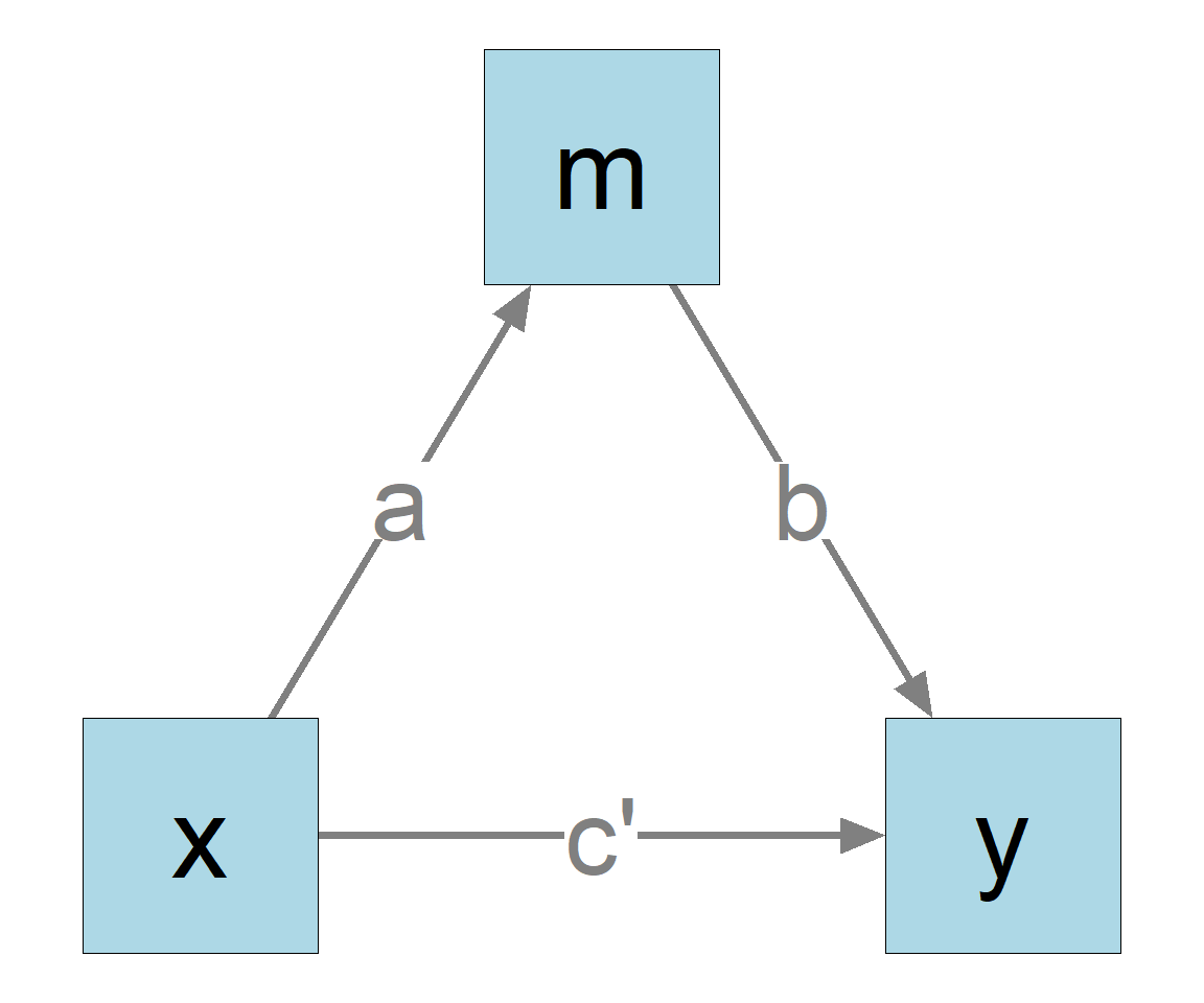
In this model:

x is the predictor (independent variable).
y is the outcome variable (dependent variable).
m is the mediator.

The goal is to compute and test the indirect effect from x to y through m.

Fit the Models by `lm()`

To estimate all the regression coefficients, just fit two regression models:

Predict m by x (Figure 2).
Predict y by m and x (Figure 3).

This can be easily done by lm() in R:

# Predict m
model_m <- lm(m ~ x,
              data = data_med)
# Predict y
model_y <- lm(y ~ m + x,
              data = data_med)

These are the regression results:

summary(model_m)

Call:
lm(formula = m ~ x, data = data_med)

Coefficients:
            Estimate Std. Error t value Pr(>|t|)    
(Intercept)  9.39332    0.83320   11.27   <2e-16 ***
x            0.92400    0.08358   11.06   <2e-16 ***
---
Signif. codes:  0 '***' 0.001 '**' 0.01 '*' 0.05 '.' 0.1 ' ' 1

Residual standard error: 0.8774 on 98 degrees of freedom
Multiple R-squared:  0.555, Adjusted R-squared:  0.5505 
F-statistic: 122.2 on 1 and 98 DF,  p-value: < 2.2e-16

summary(model_y)

Call:
lm(formula = y ~ m + x, data = data_med)

Coefficients:
            Estimate Std. Error t value Pr(>|t|)    
(Intercept)   3.3618     2.9480   1.140 0.256930    
m             0.8596     0.2358   3.645 0.000432 ***
x             0.4277     0.2925   1.462 0.146862    
---
Signif. codes:  0 '***' 0.001 '**' 0.01 '*' 0.05 '.' 0.1 ' ' 1

Residual standard error: 2.048 on 97 degrees of freedom
Multiple R-squared:  0.3512,    Adjusted R-squared:  0.3378 
F-statistic: 26.26 on 2 and 97 DF,  p-value: 7.704e-10

The direct effect is the coefficient of x in the model predicting y, which is 0.428, and not significant.

The Indirect Effect

The indirect effect is the product of the a-path and the b-path. To test this indirect effect, one common method is nonparametric bootstrapping MacKinnon et al. (2002). This can be done easily by indirect_effect() from the package manymome.

Combine the Regression Results

We first combine the regression models by lm2list() into one object to represent the whole model (Figure 1):¹

full_model <- lm2list(model_m,
                      model_y)
full_model


The models:
m ~ x
y ~ m + x

Compute and Test the Indirect Effect

For this simple model, we can simply use indirect_effect()

ind <- indirect_effect(x = "x",
                       y = "y",
                       m = "m",
                       fit = full_model,
                       boot_ci = TRUE,
                       R = 5000,
                       seed = 3456)

These are the main arguments:

x: The name of the x variable, the start of the indirect path.
y: The name of the y variable, the end of the indirect path.
m: The name of the mediator.
fit: The regression models combined by lm2list().
boot_ci: If TRUE, bootstrap confidence interval will be formed.
R, the number of bootstrap samples. It is fast for regression models and I recommend using at least 5000 bootstrap samples or even 10000, because the results may not be stable enough if indirect effect is close to zero (an example can be found in S. F. Cheung & Pesigan, 2023).
seed: The seed for the random number generator, to make the resampling reproducible. This argument should always be set when doing bootstrapping.

By default, parallel processing will be used and a progress bar will be displayed.

Just typing the name of the output can print the major results

ind


== Indirect Effect  ==
                                     
 Path:               x -> m -> y     
 Indirect Effect:    0.794           
 95.0% Bootstrap CI: [0.393 to 1.250]

Computation Formula:
  (b.m~x)*(b.y~m)
Computation:
  (0.92400)*(0.85957)

Percentile confidence interval formed by nonparametric bootstrapping
with 5000 bootstrap samples.

Coefficients of Component Paths:
 Path Coefficient
  m~x       0.924
  y~m       0.860

As shown above, the indirect effect is 0.794. The 95% bootstrap confidence interval is [0.393; 1.250]. The indirect effect is positive and significant.

For transparency, the output also shows how the indirect effect was computed.

Standardized Indirect Effect

To compute and test the standardized indirect effect, with both the x-variable and y-variable standardized, add standardized_x = TRUE and standardized_y = TRUE:

ind_stdxy <- indirect_effect(x = "x",
                             y = "y",
                             m = "m",
                             fit = full_model,
                             boot_ci = TRUE,
                             R = 5000,
                             seed = 3456,,
                             standardized_x = TRUE,
                             standardized_y = TRUE)

The results can be printed as usual:

ind_stdxy


== Indirect Effect (Both 'x' and 'y' Standardized) ==
                                     
 Path:               x -> m -> y     
 Indirect Effect:    0.333           
 95.0% Bootstrap CI: [0.170 to 0.512]

Computation Formula:
  (b.m~x)*(b.y~m)*sd_x/sd_y
Computation:
  (0.92400)*(0.85957)*(1.05515)/(2.51729)

Percentile confidence interval formed by nonparametric bootstrapping
with 5000 bootstrap samples.

Coefficients of Component Paths:
 Path Coefficient
  m~x       0.924
  y~m       0.860

NOTE:
- The effects of the component paths are from the model, not
  standardized.

The standardized indirect effect is 0.333. The 95% bootstrap confidence interval is [0.170; 0.512], significant.

A Simple Mediation Model With Some Control Variables

Suppose we want to fit a more complicated model, with some other variables included, such as control variables c1 and c2 in the dataset (Figure 4).

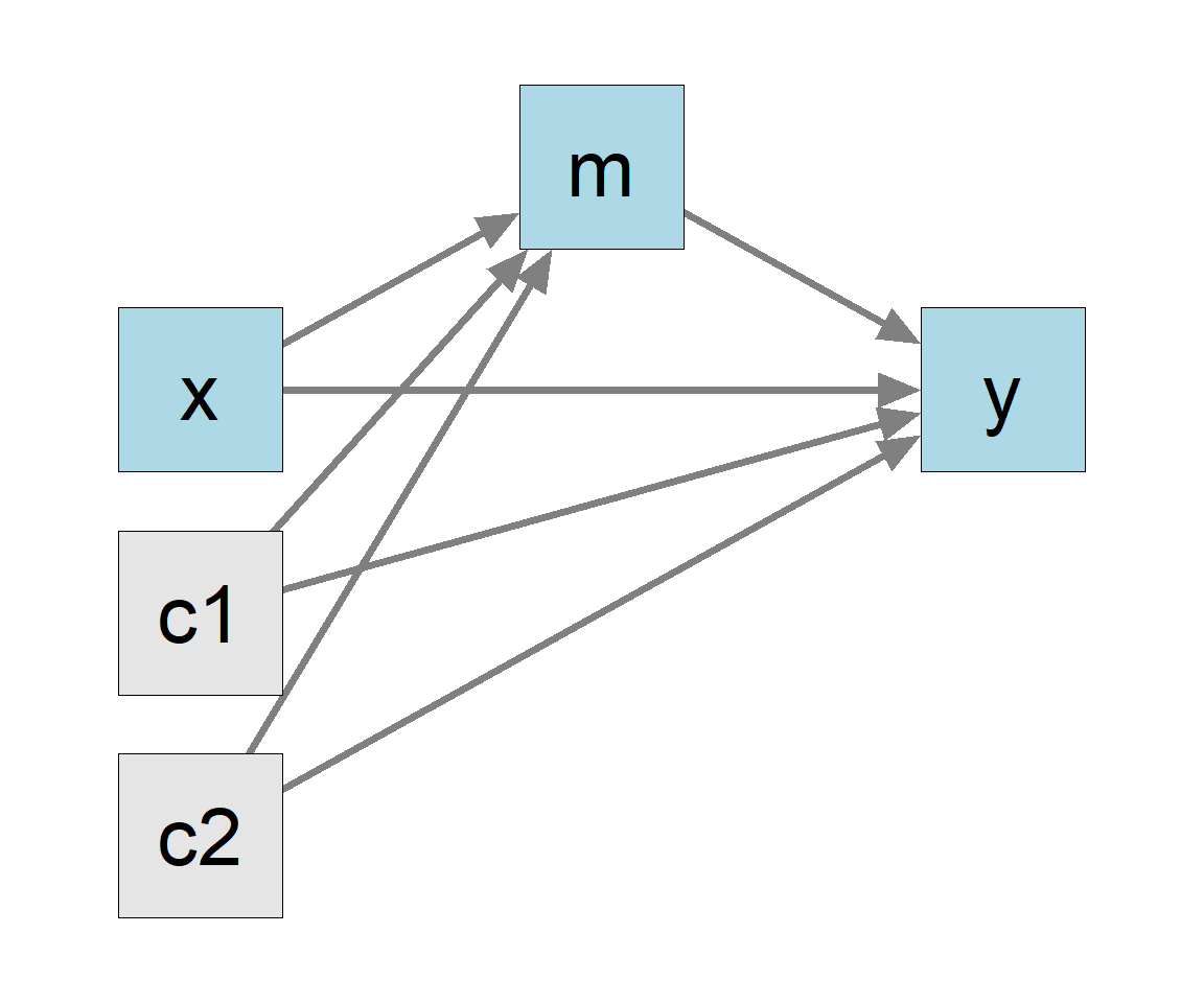
Although there are more predictors (c1 and c2) and more direct and indirect paths (e.g., c1 to y through m), there are still only just two regression models. We can fit them as usual by lm():

model2_m <- lm(m ~ x + c1 + c2,
               data = data_med)
model2_y <- lm(y ~ m + x + c1 + c2,
               data = data_med)

These are the regression results:

summary(model2_m)

Call:
lm(formula = m ~ x + c1 + c2, data = data_med)

Coefficients:
            Estimate Std. Error t value Pr(>|t|)    
(Intercept)  9.68941    0.91979  10.534   <2e-16 ***
x            0.93469    0.08083  11.563   <2e-16 ***
c1           0.19778    0.07678   2.576   0.0115 *  
c2          -0.16841    0.10305  -1.634   0.1055    
---
Signif. codes:  0 '***' 0.001 '**' 0.01 '*' 0.05 '.' 0.1 ' ' 1

Residual standard error: 0.8425 on 96 degrees of freedom
Multiple R-squared:  0.5981,    Adjusted R-squared:  0.5855 
F-statistic: 47.62 on 3 and 96 DF,  p-value: < 2.2e-16

summary(model2_y)

Call:
lm(formula = y ~ m + x + c1 + c2, data = data_med)

Coefficients:
            Estimate Std. Error t value Pr(>|t|)   
(Intercept)   4.4152     3.3016   1.337  0.18432   
m             0.7847     0.2495   3.145  0.00222 **
x             0.5077     0.3057   1.661  0.10004   
c1            0.1405     0.1941   0.724  0.47093   
c2           -0.1544     0.2554  -0.604  0.54695   
---
Signif. codes:  0 '***' 0.001 '**' 0.01 '*' 0.05 '.' 0.1 ' ' 1

Residual standard error: 2.06 on 95 degrees of freedom
Multiple R-squared:  0.3576,    Adjusted R-squared:  0.3305

We then just combine them by lm2list():

full_model2 <- lm2list(model2_m,
                       model2_y)
full_model2


The models:
m ~ x + c1 + c2
y ~ m + x + c1 + c2

The indirect effect can be computed and tested in exactly the same way:

ind2 <- indirect_effect(x = "x",
                        y = "y",
                        m = "m",
                        fit = full_model2,
                        boot_ci = TRUE,
                        R = 5000,
                        seed = 3456)

This is the result:

ind2


== Indirect Effect  ==
                                     
 Path:               x -> m -> y     
 Indirect Effect:    0.733           
 95.0% Bootstrap CI: [0.288 to 1.203]

Computation Formula:
  (b.m~x)*(b.y~m)
Computation:
  (0.93469)*(0.78469)

Percentile confidence interval formed by nonparametric bootstrapping
with 5000 bootstrap samples.

Coefficients of Component Paths:
 Path Coefficient
  m~x       0.935
  y~m       0.785

The indirect effect is 0.733. The 95% bootstrap confidence interval is [0.288; 1.203], decreased after the control variables are included, but still significant.

Standardized indirect effect can also be computed and tested just by adding standardized_x = TRUE and standardized_y = TRUE.

Advanced Topics

Customize the Printout

The printout can be customized in several ways. For example:

print(ind,
      digits = 2,
      pvalue = TRUE,
      pvalue_digits = 3,
      se = TRUE)


== Indirect Effect  ==
                                   
 Path:               x -> m -> y   
 Indirect Effect:    0.79          
 95.0% Bootstrap CI: [0.39 to 1.25]
 Bootstrap p-value:  0.000         
 Bootstrap SE:       0.22          

Computation Formula:
  (b.m~x)*(b.y~m)
Computation:
  (0.92400)*(0.85957)

Percentile confidence interval formed by nonparametric bootstrapping
with 5000 bootstrap samples.
Standard error (SE) based on nonparametric bootstrapping with 5000
bootstrap samples.

Coefficients of Component Paths:
 Path Coefficient
  m~x        0.92
  y~m        0.86

digits: The number of digits after the decimal point for major output. Default is 3.
pvalue: Whether bootstrapping p-value is printed. The method by Asparouhov & Muthén (2021) is used.
pvalue_digits: The number of digits after the decimal point for the p-value. Default is 3.
se: The standard error based on bootstrapping (i.e., the standard deviation of the bootstrap estimates).

Missing Data

Care needs to be taken if missing data is present. Let’s remove some data points from the data file:

data_med_missing <- data_med
data_med_missing[1:3, "x"] <- NA
data_med_missing[2:4, "m"] <- NA
data_med_missing[3:6, "y"] <- NA
head(data_med_missing)

          x        m        y       c1       c2
1        NA 17.89644 20.73893 1.426513 6.103290
2        NA       NA 22.91594 2.940388 3.832698
3        NA       NA       NA 3.012678 5.770532
4 11.196969       NA       NA 3.120056 4.654931
5 11.887811 22.08645       NA 4.440018 3.959033
6  8.198297 16.95198       NA 2.495083 3.763712

If we do the regression separately, the cases used in the two models will be different:

# Predict m
model_m_missing <- lm(m ~ x,
                      data = data_med_missing)
# Predict y
model_y_missing <- lm(y ~ m + x,
                      data = data_med_missing)

The sample sizes are not the same:

nobs(model_m_missing)

[1] 96

nobs(model_y_missing)

[1] 94

If they are combined by lm2list(), an error will occur. The function lm2list() will compare the data to see if the cases used are likely to be different.²

lm2list(model_m_missing,
        model_y_missing)

Error in check_lm_consistency(...): The data sets used in the lm models do not have identical sample size. All lm models must be fitted to the same sample.

A simple (though not ideal) solution is to use listwise deletion, keeping only cases with complete data. This can be done by na.omit():

data_med_listwise <- na.omit(data_med_missing)
head(data_med_listwise)

           x        m        y         c1       c2
7  10.091769 19.42649 26.14005  2.5023227 6.196603
8   9.307707 18.29251 24.24033  1.3108621 4.892843
9   6.904119 15.91634 23.97662  1.3010467 3.796913
10 10.706891 18.00798 26.55098  1.9488566 5.835160
11  9.524557 17.80304 24.14855 -0.4604918 3.663987
12  9.307470 17.21214 23.17019  4.2970431 5.538241

nrow(data_med_listwise)

[1] 94

The number of cases using listwise deletion is 94, less than the full sample with missing data (100).

The steps above can then be proceed as usual.

Functions Used In This Example

These are the main functions used:

lm2list(): Combining the results of several one-outcome regression models.
indirect_effect(): Compute and test an indirect effect.

Further Information

The package manymome has no inherent limitations on the number of variables and the form of the mediation models. An illustration using a more complicated models with both parallel and serial mediation paths can be found in this online article.

Other features of manymome can be found in the website for it.

Disclaimer: Similarity Across Tutorials

To keep each tutorial self-contained, some sections are intentionally repeated nearly verbatim (“recycled”) to reduce the hassle to read several articles to learn how to do one task.

Revision History and Issues

The revision history of this post can be find in the GitHub history of the source file.

For issues on this post, such as corrections and mistakes, please open an issue for the GitHub repository for this blog. Thanks.

:::

References

Asparouhov, T., & Muthén, B. O. (2021). Bootstrap p-value computation. https://www.statmodel.com/download/FAQ-Bootstrap%20-%20Pvalue.pdf

Cheung, M. W.-L. (2009). Comparison of methods for constructing confidence intervals of standardized indirect effects. Behavior Research Methods, 41(2), 425–438. https://doi.org/10.3758/BRM.41.2.425

Cheung, S. F., & Cheung, S.-H. (2024). Manymome: An R package for computing the indirect effects, conditional effects, and conditional indirect effects, standardized or unstandardized, and their bootstrap confidence intervals, in many (though not all) models. Behavior Research Methods, 56(5), 4862–4882. https://doi.org/10.3758/s13428-023-02224-z

Cheung, S. F., & Pesigan, I. J. A. (2023). Semlbci: An R package for forming likelihood-based confidence intervals for parameter estimates, correlations, indirect effects, and other derived parameters. Structural Equation Modeling: A Multidisciplinary Journal, 30(6), 985–999. https://doi.org/10.1080/10705511.2023.2183860

MacKinnon, D. P., Lockwood, C. M., Hoffman, J. M., West, S. G., & Sheets, V. (2002). A comparison of methods to test mediation and other intervening variable effects. Psychological Methods, 7(1), 83–104. http://www.ncbi.nlm.nih.gov/pmc/articles/PMC2819363/

Footnotes

The order does not matter when using lm2list.↩︎
The function lm2list() checks not only sample sizes. Even if the sample sizes are the same, an error will still be raised if there is evidence suggesting that the samples are not the same, such as different values of x in the two models.↩︎