This tutorial shows how to use the R package manymome (S. F. Cheung & Cheung, 2024), a flexible package for mediation analysis, to test indirect effects in a serial mediation model fitted by multiple regression.

Pre-Requisite

Readers are expected to have basic R skills and know how to fit a linear regression model using lm().

The package manymome can be installed from CRAN:

install.packages("manymome")

Data

This is the data file for illustration, from manymome:

library(manymome)
head(data_serial, 3)

          x       m1        m2         y         c1       c2
1 12.123280 20.57654  9.327606  9.002655  0.1092621 6.011779
2  9.811849 18.20839  9.467283 11.561813 -0.1240136 6.423912
3 10.111538 20.34305 10.054767  9.348610  4.2786083 5.336944

A Serial Mediation Model

First we fit a serial mediation model using only x, m1, m2, and y.

In this model:

x is the predictor (independent variable).
y is the outcome variable (dependent variable).
m1 and m2 are the mediators.

The goal is to compute and test the following indirect effects from x to y:

x -> m1 -> m2 -> y.
x -> m1 -> y.
x -> m2 -> y.

Fit the Models by `lm()`

To estimate all the regression coefficients, just fit three regression models:

Predict m1 by x (Figure 2).
Predict m2 by m1 and x (Figure 3).
Predict y by m1, m2, and x (Figure 4).

This can be easily done by lm() in R:

# Predict m1
model_m1 <- lm(m1 ~ x,
               data = data_serial)
# Predict m2
model_m2 <- lm(m2 ~ m1 + x,
               data = data_serial)
# Predict y
model_y <- lm(y ~ m2 + m1 + x,
              data = data_serial)

These are the regression results:

summary(model_m1)

Call:
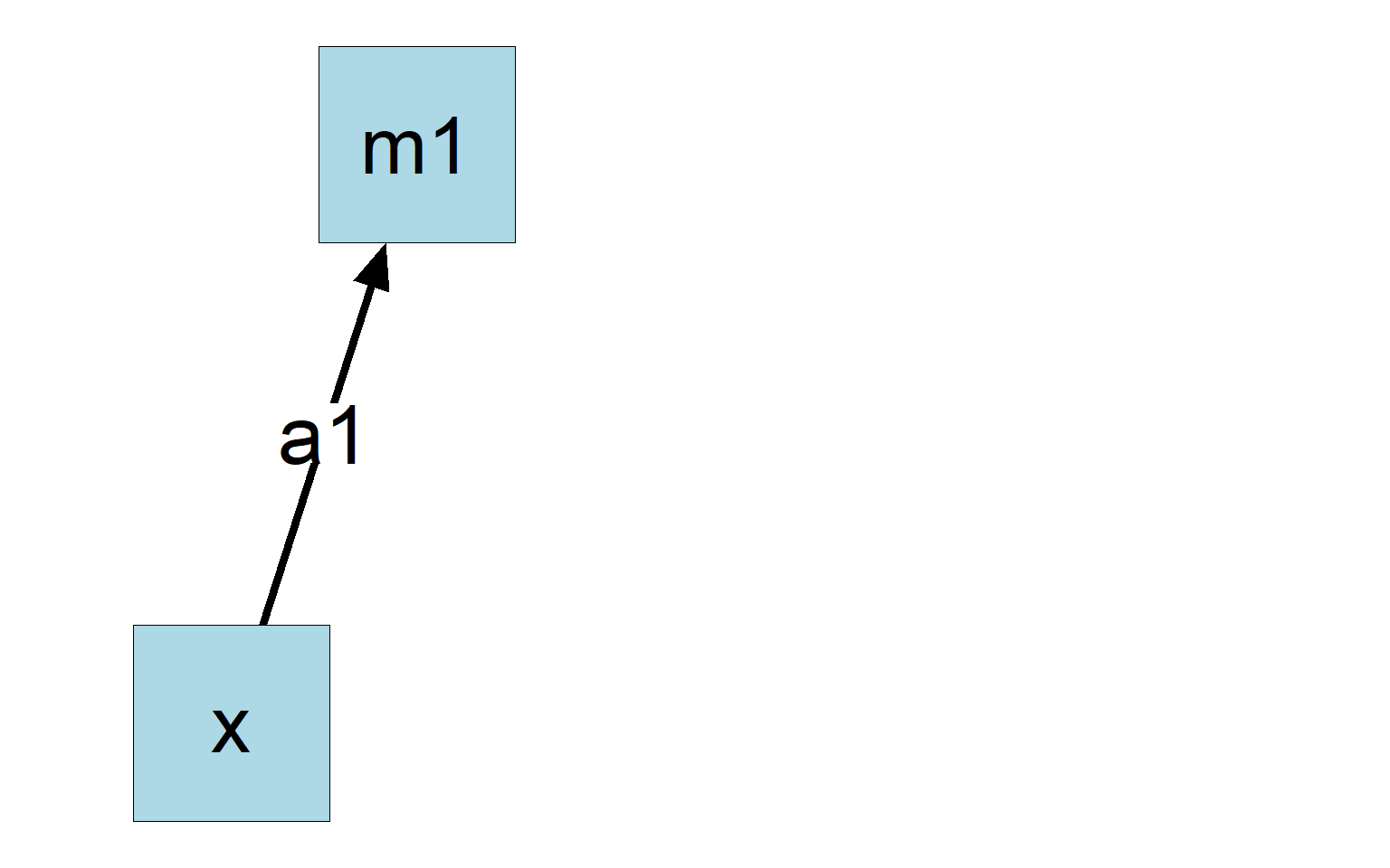
lm(formula = m1 ~ x, data = data_serial)

Coefficients:
            Estimate Std. Error t value Pr(>|t|)    
(Intercept) 10.15035    0.97278  10.434  < 2e-16 ***
x            0.82684    0.09694   8.529 1.86e-13 ***
---
Signif. codes:  0 '***' 0.001 '**' 0.01 '*' 0.05 '.' 0.1 ' ' 1

Residual standard error: 0.9211 on 98 degrees of freedom
Multiple R-squared:  0.4261,    Adjusted R-squared:  0.4202 
F-statistic: 72.75 on 1 and 98 DF,  p-value: 1.86e-13

summary(model_m2)

Call:
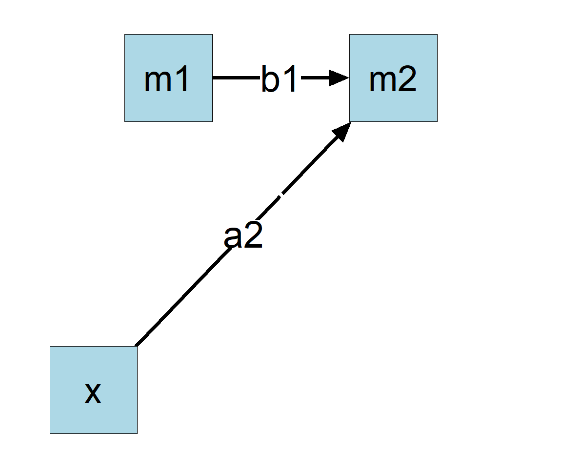
lm(formula = m2 ~ m1 + x, data = data_serial)

Coefficients:
            Estimate Std. Error t value Pr(>|t|)    
(Intercept)   2.2075     1.4396   1.533    0.128    
m1            0.5295     0.1029   5.146 1.39e-06 ***
x            -0.2122     0.1303  -1.628    0.107    
---
Signif. codes:  0 '***' 0.001 '**' 0.01 '*' 0.05 '.' 0.1 ' ' 1

Residual standard error: 0.9382 on 97 degrees of freedom
Multiple R-squared:  0.2463,    Adjusted R-squared:  0.2307

summary(model_y)

Call:
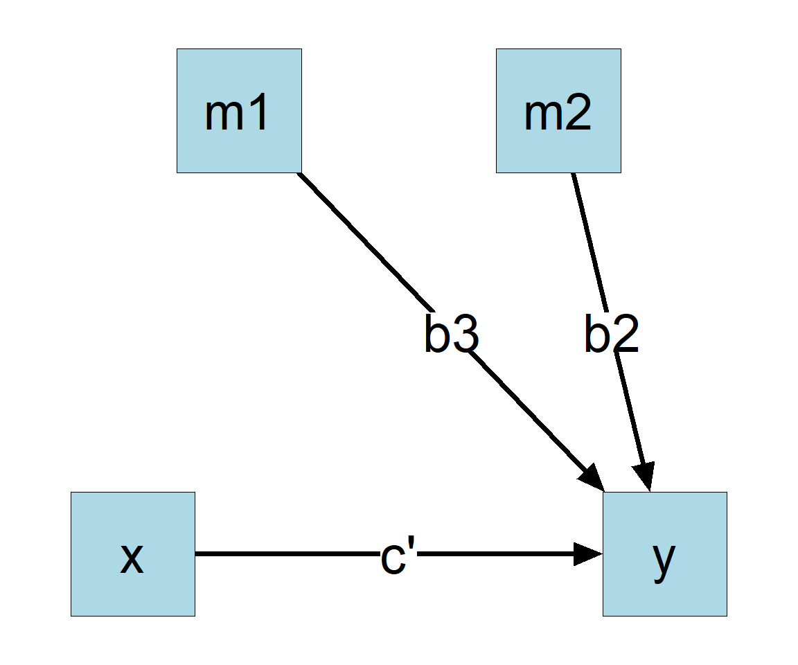
lm(formula = y ~ m2 + m1 + x, data = data_serial)

Coefficients:
            Estimate Std. Error t value Pr(>|t|)   
(Intercept)   8.5543     3.0282   2.825  0.00575 **
m2            0.5736     0.2110   2.718  0.00779 **
m1           -0.4149     0.2413  -1.720  0.08870 . 
x             0.4654     0.2746   1.695  0.09331 . 
---
Signif. codes:  0 '***' 0.001 '**' 0.01 '*' 0.05 '.' 0.1 ' ' 1

Residual standard error: 1.95 on 96 degrees of freedom
Multiple R-squared:  0.08713,   Adjusted R-squared:  0.05861 
F-statistic: 3.054 on 3 and 96 DF,  p-value: 0.03212

The direct effect is the coefficient of x in the model predicting y, which is 0.465, and not significant.

The Indirect Effects

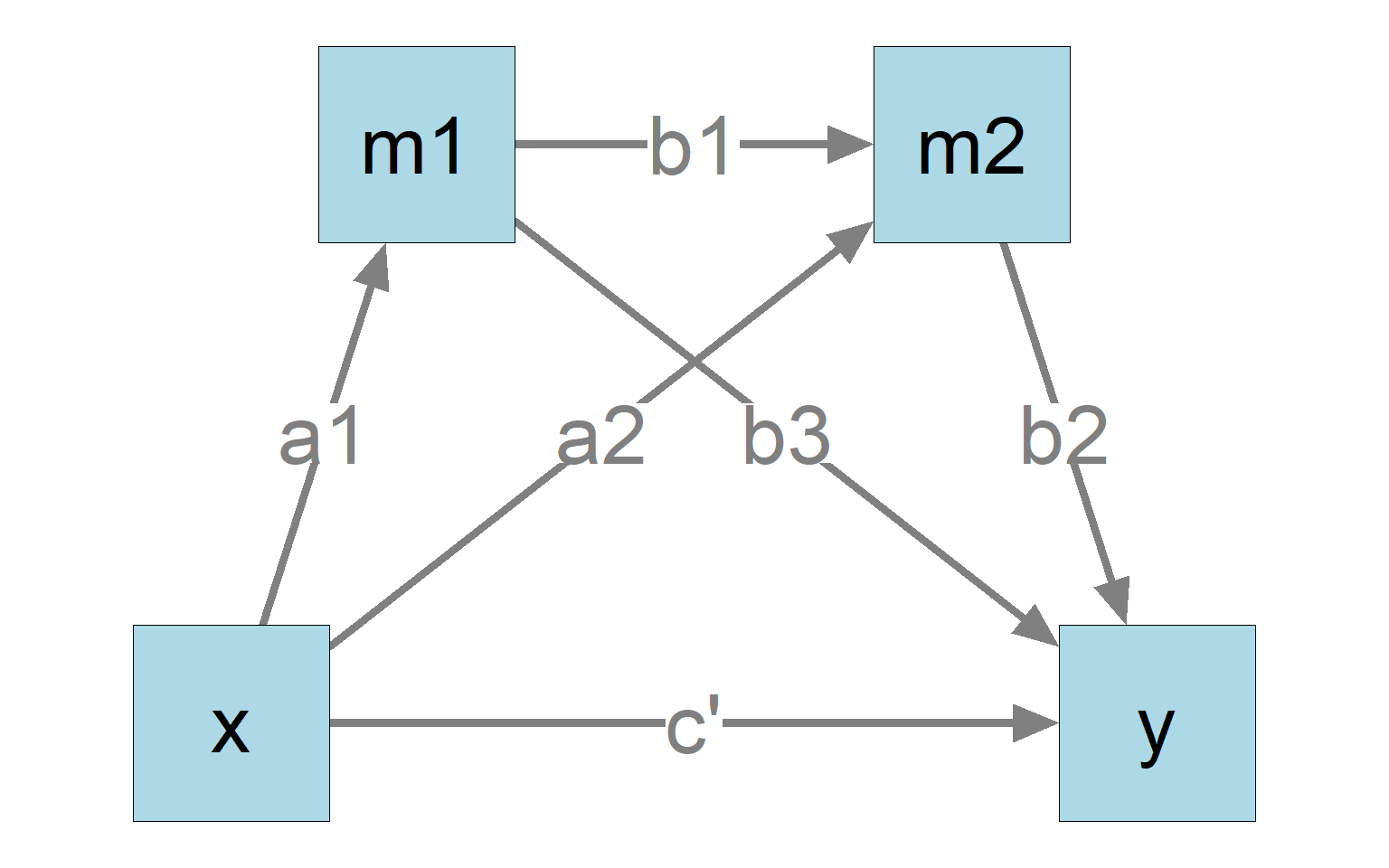
The three indirect effects are computed from the products:

x -> m1 -> m2 -> y
- The product of a1-path, b1-path, and b2-path.
x -> m1 -> y
- The product of a1-path and b3-path.
x -> m2 -> y
- The product of a2-path and b2-path.

To test these indirect effects, one common method is nonparametric bootstrapping MacKinnon et al. (2002). This can be done easily by indirect_effect() from the package manymome.

Combine the Regression Results

We first combine the regression models by lm2list() into one object to represent the whole model (Figure 1):¹

full_model <- lm2list(model_m1,
                      model_m2,
                      model_y)
full_model


The models:
m1 ~ x
m2 ~ m1 + x
y ~ m2 + m1 + x

Compute and Test the Indirect Effect

For this serial mediation model, we can simply use indirect_effect()

ind12 <- indirect_effect(x = "x",
                         y = "y",
                         m = c("m1", "m2"),
                         fit = full_model,
                         boot_ci = TRUE,
                         R = 5000,
                         seed = 3456)

These are the main arguments:

x: The name of the x variable, the start of the indirect path.
y: The name of the y variable, the end of the indirect path.
m: A character vector of the names of the mediators. The path goes from the first name to the last name. In the example above, the path is x -> m1 -> m2 -> y. Therefore, m is set to c("m1", "m2").
fit: The regression models combined by lm2list().
boot_ci: If TRUE, bootstrap confidence interval will be formed.
R, the number of bootstrap samples. It is fast for regression models and I recommend using at least 5000 bootstrap samples or even 10000, because the results may not be stable enough if indirect effect is close to zero (an example can be found in S. F. Cheung & Pesigan, 2023).
seed: The seed for the random number generator, to make the resampling reproducible. This argument should always be set when doing bootstrapping.

By default, parallel processing will be used and a progress bar will be displayed.

ind1 <- indirect_effect(x = "x",
                        y = "y",
                        m = "m1",
                        fit = full_model,
                        boot_ci = TRUE,
                        R = 5000,
                        seed = 3456)

ind2 <- indirect_effect(x = "x",
                        y = "y",
                        m = "m2",
                        fit = full_model,
                        boot_ci = TRUE,
                        R = 5000,
                        seed = 3456)

Just typing the name of the output can print the major results

ind12


== Indirect Effect  ==
                                       
 Path:               x -> m1 -> m2 -> y
 Indirect Effect:    0.251             
 95.0% Bootstrap CI: [0.075 to 0.500]  

Computation Formula:
  (b.m1~x)*(b.m2~m1)*(b.y~m2)
Computation:
  (0.82684)*(0.52946)*(0.57361)

Percentile confidence interval formed by nonparametric bootstrapping
with 5000 bootstrap samples.

Coefficients of Component Paths:
  Path Coefficient
  m1~x       0.827
 m2~m1       0.529
  y~m2       0.574

ind1


== Indirect Effect  ==
                                       
 Path:               x -> m1 -> y      
 Indirect Effect:    -0.343            
 95.0% Bootstrap CI: [-0.672 to -0.015]

Computation Formula:
  (b.m1~x)*(b.y~m1)
Computation:
  (0.82684)*(-0.41495)

Percentile confidence interval formed by nonparametric bootstrapping
with 5000 bootstrap samples.

Coefficients of Component Paths:
 Path Coefficient
 m1~x       0.827
 y~m1      -0.415

ind2


== Indirect Effect  ==
                                      
 Path:               x -> m2 -> y     
 Indirect Effect:    -0.122           
 95.0% Bootstrap CI: [-0.376 to 0.055]

Computation Formula:
  (b.m2~x)*(b.y~m2)
Computation:
  (-0.21223)*(0.57361)

Percentile confidence interval formed by nonparametric bootstrapping
with 5000 bootstrap samples.

Coefficients of Component Paths:
 Path Coefficient
 m2~x      -0.212
 y~m2       0.574

As shown above, the indirect effect through m1 and then m2 is 0.251. The 95% bootstrap confidence interval is [0.075; 0.500]. The indirect effect is positive and significant.

The indirect effect through m1 only is -0.343. The 95% bootstrap confidence interval is [-0.672; -0.015]. The indirect effect is negative and significant.

The indirect effect through m2 only is -0.122. The 95% bootstrap confidence interval is [-0.376; 0.055]. The indirect effect is not significant.

For transparency, the output also shows how the indirect effect was computed.

Standardized Indirect Effect

To compute and test the standardized indirect effects, with both the x-variable and y-variable standardized, add standardized_x = TRUE and standardized_y = TRUE:

ind12_stdxy <- indirect_effect(x = "x",
                               y = "y",
                               m = c("m1", "m2"),
                               fit = full_model,
                               boot_ci = TRUE,
                               R = 5000,
                               seed = 3456,
                               standardized_x = TRUE,
                               standardized_y = TRUE)
ind1_stdxy <- indirect_effect(x = "x",
                              y = "y",
                              m = "m1",
                              fit = full_model,
                              boot_ci = TRUE,
                              R = 5000,
                              seed = 3456,
                              standardized_x = TRUE,
                              standardized_y = TRUE)
ind2_stdxy <- indirect_effect(x = "x",
                              y = "y",
                              m = "m2",
                              fit = full_model,
                              boot_ci = TRUE,
                              R = 5000,
                              seed = 3456,
                              standardized_x = TRUE,
                              standardized_y = TRUE)

The results can be printed as usual:

ind12_stdxy


== Indirect Effect (Both 'x' and 'y' Standardized) ==
                                       
 Path:               x -> m1 -> m2 -> y
 Indirect Effect:    0.119             
 95.0% Bootstrap CI: [0.038 to 0.228]  

Computation Formula:
  (b.m1~x)*(b.m2~m1)*(b.y~m2)*sd_x/sd_y
Computation:
  (0.82684)*(0.52946)*(0.57361)*(0.95489)/(2.00967)

Percentile confidence interval formed by nonparametric bootstrapping
with 5000 bootstrap samples.

Coefficients of Component Paths:
  Path Coefficient
  m1~x       0.827
 m2~m1       0.529
  y~m2       0.574

NOTE:
- The effects of the component paths are from the model, not
  standardized.

ind1_stdxy


== Indirect Effect (Both 'x' and 'y' Standardized) ==
                                       
 Path:               x -> m1 -> y      
 Indirect Effect:    -0.163            
 95.0% Bootstrap CI: [-0.317 to -0.008]

Computation Formula:
  (b.m1~x)*(b.y~m1)*sd_x/sd_y
Computation:
  (0.82684)*(-0.41495)*(0.95489)/(2.00967)

Percentile confidence interval formed by nonparametric bootstrapping
with 5000 bootstrap samples.

Coefficients of Component Paths:
 Path Coefficient
 m1~x       0.827
 y~m1      -0.415

NOTE:
- The effects of the component paths are from the model, not
  standardized.

ind2_stdxy


== Indirect Effect (Both 'x' and 'y' Standardized) ==
                                      
 Path:               x -> m2 -> y     
 Indirect Effect:    -0.058           
 95.0% Bootstrap CI: [-0.176 to 0.025]

Computation Formula:
  (b.m2~x)*(b.y~m2)*sd_x/sd_y
Computation:
  (-0.21223)*(0.57361)*(0.95489)/(2.00967)

Percentile confidence interval formed by nonparametric bootstrapping
with 5000 bootstrap samples.

Coefficients of Component Paths:
 Path Coefficient
 m2~x      -0.212
 y~m2       0.574

NOTE:
- The effects of the component paths are from the model, not
  standardized.

The standardized indirect effect through m1 and then m2 is 0.119. The 95% bootstrap confidence interval is [0.038; 0.228], significant.

The standardized indirect effect through m1 is -0.163. The 95% bootstrap confidence interval is [-0.317; -0.008], negative and significant.

The standardized indirect effect through m2 is -0.058. The 95% bootstrap confidence interval is [-0.176; 0.025], not significant.

Total Indirect Effect

Suppose we would like to compute the total indirect effects from x to y through all the paths involving m1 and m2. This can be done by “adding” the indirect effects computed above, simply by using the + operator:

ind_total <- ind12 + ind1 + ind2

ind_total


== Indirect Effect  ==
                                        
 Path:                x -> m1 -> m2 -> y
 Path:                x -> m1 -> y      
 Path:                x -> m2 -> y      
 Function of Effects: -0.214            
 95.0% Bootstrap CI:  [-0.541 to 0.093] 

Computation of the Function of Effects:
 ((x->m1->m2->y)
+(x->m1->y))
+(x->m2->y) 


Percentile confidence interval formed by nonparametric bootstrapping
with 5000 bootstrap samples.

The standardized total indirect effect can be computed similarly:

ind_total_stdxy <- ind12_stdxy + ind1_stdxy + ind2_stdxy

ind_total_stdxy


== Indirect Effect (Both 'x' and 'y' Standardized) ==
                                        
 Path:                x -> m1 -> m2 -> y
 Path:                x -> m1 -> y      
 Path:                x -> m2 -> y      
 Function of Effects: -0.102            
 95.0% Bootstrap CI:  [-0.262 to 0.043] 

Computation of the Function of Effects:
 ((x->m1->m2->y)
+(x->m1->y))
+(x->m2->y) 


Percentile confidence interval formed by nonparametric bootstrapping
with 5000 bootstrap samples.

The total indirect effect is not significant in this example. Nevertheless, this should be interpreted with cautions because the paths are not of the same sign, some positive and some negative. This is an example of inconsistent mediation.

A Serial Mediation Model With Some Control Variables

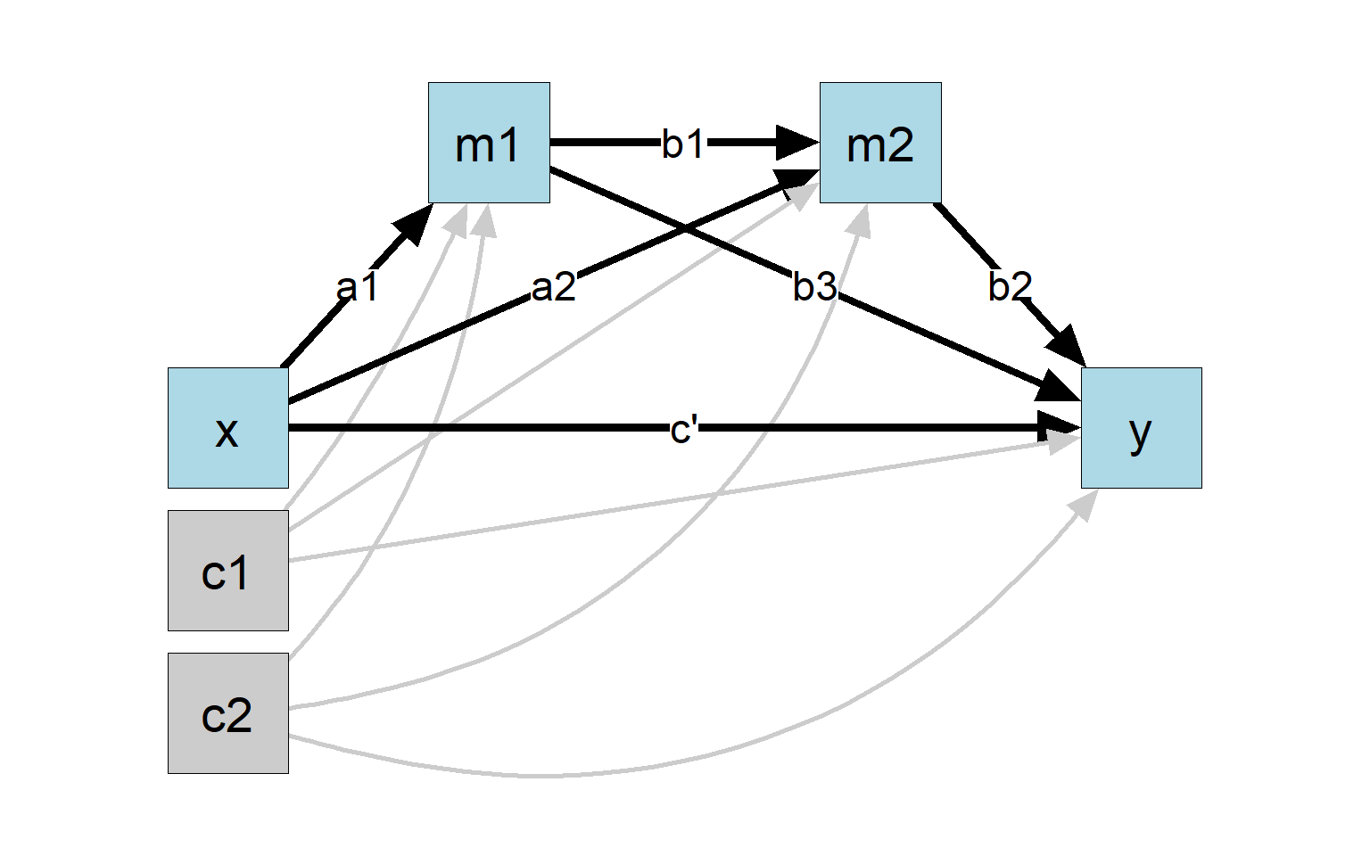
Suppose we want to fit a more complicated model, with some other variables included, such as control variables c1 and c2 in the dataset (Figure 5).

Although there are more predictors (c1 and c2) and more direct and indirect paths (e.g., c1 to y through m1), there are still only just three regression models. We can fit them as usual by lm():

model2_m1 <- lm(m1 ~ x + c1 + c2,
                data = data_serial)
model2_m2 <- lm(m2 ~ m1 + x + c1 + c2,
                data = data_serial)
model2_y <- lm(y ~ m1 + m2 + x + c1 + c2,
               data = data_serial)

These are the regression results:

summary(model2_m1)

Call:
lm(formula = m1 ~ x + c1 + c2, data = data_serial)

Coefficients:
            Estimate Std. Error t value Pr(>|t|)    
(Intercept) 10.81566    1.14379   9.456 2.20e-15 ***
x            0.82244    0.09424   8.727 8.03e-14 ***
c1           0.17148    0.09070   1.891   0.0617 .  
c2          -0.18886    0.09278  -2.036   0.0446 *  
---
Signif. codes:  0 '***' 0.001 '**' 0.01 '*' 0.05 '.' 0.1 ' ' 1

Residual standard error: 0.888 on 96 degrees of freedom
Multiple R-squared:  0.4774,    Adjusted R-squared:  0.4611 
F-statistic: 29.23 on 3 and 96 DF,  p-value: 1.629e-13

summary(model2_m2)

Call:
lm(formula = m2 ~ m1 + x + c1 + c2, data = data_serial)

Coefficients:
            Estimate Std. Error t value Pr(>|t|)    
(Intercept)  3.51937    1.58681   2.218  0.02895 *  
m1           0.42078    0.10188   4.130  7.8e-05 ***
x           -0.11610    0.12598  -0.922  0.35909    
c1           0.27753    0.09221   3.010  0.00335 ** 
c2          -0.16195    0.09460  -1.712  0.09017 .  
---
Signif. codes:  0 '***' 0.001 '**' 0.01 '*' 0.05 '.' 0.1 ' ' 1

Residual standard error: 0.8864 on 95 degrees of freedom
Multiple R-squared:  0.341, Adjusted R-squared:  0.3133

summary(model2_y)

Call:
lm(formula = y ~ m1 + m2 + x + c1 + c2, data = data_serial)

Coefficients:
            Estimate Std. Error t value Pr(>|t|)  
(Intercept)  9.46788    3.60900   2.623   0.0102 *
m1          -0.43534    0.24539  -1.774   0.0793 .
m2           0.52077    0.22753   2.289   0.0243 *
x            0.49285    0.28063   1.756   0.0823 .
c1           0.09884    0.21403   0.462   0.6453  
c2          -0.09604    0.21300  -0.451   0.6531  
---
Signif. codes:  0 '***' 0.001 '**' 0.01 '*' 0.05 '.' 0.1 ' ' 1

Residual standard error: 1.966 on 94 degrees of freedom
F-statistic: 1.893 on 5 and 94 DF,  p-value: 0.1028

We then just combine them by lm2list():

full_model2 <- lm2list(model2_m1,
                       model2_m2,
                       model2_y)
full_model2


The models:
m1 ~ x + c1 + c2
m2 ~ m1 + x + c1 + c2
y ~ m1 + m2 + x + c1 + c2

The indirect effects can be computed and tested in exactly the same way:

ind2_12 <- indirect_effect(x = "x",
                           y = "y",
                           m = c("m1", "m2"),
                           fit = full_model2,
                           boot_ci = TRUE,
                           R = 5000,
                           seed = 3456)

ind2_1 <- indirect_effect(x = "x",
                          y = "y",
                          m = "m1",
                          fit = full_model2,
                          boot_ci = TRUE,
                          R = 5000,
                          seed = 3456)

ind2_2 <- indirect_effect(x = "x",
                          y = "y",
                          m = "m2",
                          fit = full_model2,
                          boot_ci = TRUE,
                          R = 5000,
                          seed = 3456)

This is the result:

ind2_12


== Indirect Effect  ==
                                       
 Path:               x -> m1 -> m2 -> y
 Indirect Effect:    0.180             
 95.0% Bootstrap CI: [0.032 to 0.385]  

Computation Formula:
  (b.m1~x)*(b.m2~m1)*(b.y~m2)
Computation:
  (0.82244)*(0.42078)*(0.52077)

Percentile confidence interval formed by nonparametric bootstrapping
with 5000 bootstrap samples.

Coefficients of Component Paths:
  Path Coefficient
  m1~x       0.822
 m2~m1       0.421
  y~m2       0.521

ind2_1


== Indirect Effect  ==
                                       
 Path:               x -> m1 -> y      
 Indirect Effect:    -0.358            
 95.0% Bootstrap CI: [-0.704 to -0.018]

Computation Formula:
  (b.m1~x)*(b.y~m1)
Computation:
  (0.82244)*(-0.43534)

Percentile confidence interval formed by nonparametric bootstrapping
with 5000 bootstrap samples.

Coefficients of Component Paths:
 Path Coefficient
 m1~x       0.822
 y~m1      -0.435

ind2_2


== Indirect Effect  ==
                                      
 Path:               x -> m2 -> y     
 Indirect Effect:    -0.060           
 95.0% Bootstrap CI: [-0.267 to 0.099]

Computation Formula:
  (b.m2~x)*(b.y~m2)
Computation:
  (-0.11610)*(0.52077)

Percentile confidence interval formed by nonparametric bootstrapping
with 5000 bootstrap samples.

Coefficients of Component Paths:
 Path Coefficient
 m2~x      -0.116
 y~m2       0.521

The indirect effect through m1 and then m2 is 0.180. The 95% bootstrap confidence interval is [0.032; 0.385], still still significant after controlling for the effects of c1 and c2.

The indirect effect through only m1 is -0.358. The 95% bootstrap confidence interval is [-0.704; -0.018]. The indirect effect through only m2 is -0.060. The 95% bootstrap confidence interval is [-0.267; 0.099]. Both indirect effects are not significant after controlling for the effects of c1 and c2.

Standardized indirect effects can also be computed and tested just by adding standardized_x = TRUE and standardized_y = TRUE.

The total indirect effect can also be computed using +:

ind2_total <- ind2_12 + ind2_1 + ind2_2
ind2_total


== Indirect Effect  ==
                                        
 Path:                x -> m1 -> m2 -> y
 Path:                x -> m1 -> y      
 Path:                x -> m2 -> y      
 Function of Effects: -0.238            
 95.0% Bootstrap CI:  [-0.585 to 0.074] 

Computation of the Function of Effects:
 ((x->m1->m2->y)
+(x->m1->y))
+(x->m2->y) 


Percentile confidence interval formed by nonparametric bootstrapping
with 5000 bootstrap samples.

Again, this should be interpreted with cautions because the paths are not of the same sign.

No Limit On The Number of Mediators

Although the example above only has two mediators, there is no limit on the number of mediators in the serial mediation model. Just fit all the regression models predicting the mediators, combine them by lm2list(), and compute the indirect effect as illustrated above for each path.

Easy To Fit Models With Only Some Paths Included

Although x points to all m variables in the model above, and control variables predict all variables other than x, it is easy to fit a model with only paths theoretically meaningful:

Just fit the desired models by lm() and use indirect_effect() as usual.

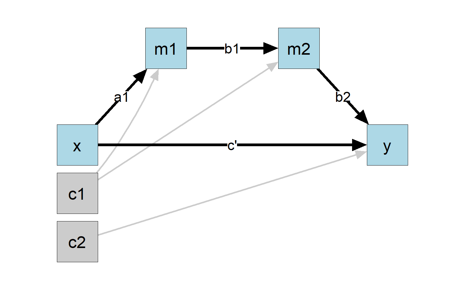
For example, suppose this is the desired model (Figure 6):

The control variable c1 only predicts m1 and m2, and the control variable c2 only predicts y, and the only indirect path is x1 -> m1 -> m2 -> y.

We just fit the three models using lm() based on the hypothesized model:

# Predict m1
model_m1 <- lm(m1 ~ x + c1,
               data = data_serial)
# Predict m2
model_m2 <- lm(m2 ~ m1 + c1,
               data = data_serial)
# Predict y
model_y <- lm(y ~ m2 + x + c2,
              data = data_serial)
# Combine the models
full_model <- lm2list(model_m1,
                      model_m2,
                      model_y)

Then the indirect effect can be computed as before.

Advanced Topics

Customize the Printout

The printout can be customized in several ways. For example:

print(ind12,
      digits = 2,
      pvalue = TRUE,
      pvalue_digits = 3,
      se = TRUE)


== Indirect Effect  ==
                                       
 Path:               x -> m1 -> m2 -> y
 Indirect Effect:    0.25              
 95.0% Bootstrap CI: [0.08 to 0.50]    
 Bootstrap p-value:  0.004             
 Bootstrap SE:       0.11              

Computation Formula:
  (b.m1~x)*(b.m2~m1)*(b.y~m2)
Computation:
  (0.82684)*(0.52946)*(0.57361)

Percentile confidence interval formed by nonparametric bootstrapping
with 5000 bootstrap samples.
Standard error (SE) based on nonparametric bootstrapping with 5000
bootstrap samples.

Coefficients of Component Paths:
  Path Coefficient
  m1~x        0.83
 m2~m1        0.53
  y~m2        0.57

digits: The number of digits after the decimal point for major output. Default is 3.
pvalue: Whether bootstrapping p-value is printed. The method by Asparouhov & Muthén (2021) is used.
pvalue_digits: The number of digits after the decimal point for the p-value. Default is 3.
se: The standard error based on bootstrapping (i.e., the standard deviation of the bootstrap estimates).

Missing Data

Care needs to be taken if missing data is present. Let’s remove some data points from the data file:

data_serial_missing <- data_serial
data_serial_missing[1:3, "x"] <- NA
data_serial_missing[2:4, "m1"] <- NA
data_serial_missing[3:5, "m2"] <- NA
data_serial_missing[3:6, "y"] <- NA
head(data_serial_missing)

          x       m1       m2         y           c1       c2
1        NA 20.57654 9.327606  9.002655  0.109262124 6.011779
2        NA       NA 9.467283 11.561813 -0.124013582 6.423912
3        NA       NA       NA        NA  4.278608266 5.336944
4 10.071555       NA       NA        NA  1.245356016 5.589547
5 11.912888 20.54746       NA        NA -0.000932131 5.339643
6  9.126304 16.53879 8.933963        NA  1.802726620 5.905691

If we do the regression separately, the cases used in the two models will be different:

# Predict m1
model_m1_missing <- lm(m1 ~ x,
                      data = data_serial_missing)
model_m2_missing <- lm(m2 ~ m1 + x,
                      data = data_serial_missing)
# Predict y
model_y_missing <- lm(y ~ m2 + m1 + x,
                      data = data_serial_missing)

The sample sizes are not the same:

nobs(model_m1_missing)

[1] 96

nobs(model_m2_missing)

[1] 95

nobs(model_y_missing)

[1] 94

If they are combined by lm2list(), an error will occur. The function lm2list() will compare the data to see if the cases used are likely to be different.²

lm2list(model_m1_missing,
        model_m2_missing,
        model_y_missing)

Error in check_lm_consistency(...): The data sets used in the lm models do not have identical sample size. All lm models must be fitted to the same sample.

A simple (though not ideal) solution is to use listwise deletion, keeping only cases with complete data. This can be done by na.omit():

data_serial_listwise <- na.omit(data_serial_missing)
head(data_serial_listwise)

           x       m1        m2         y       c1       c2
7  10.155132 17.18210  7.492526 10.621663 2.308957 5.782383
8   9.086526 18.43523  8.259809 11.947661 1.143850 5.697380
9  10.826916 19.79991 12.235185 11.118033 2.394711 4.036630
10 10.422038 17.62173 10.742770  9.863857 2.390169 5.247402
11  9.320105 18.49081 11.881927  9.730757 2.447613 4.294859
12  7.815929 16.07152  8.566832 12.520207 1.331264 4.676967

nrow(data_serial_listwise)

[1] 94

The number of cases using listwise deletion is 94, less than the full sample with missing data (94).

The steps above can then be proceed as usual.

Functions Used In This Example

These are the main functions used:

lm2list(): Combining the results of several one-outcome regression models.
indirect_effect(): Compute and test an indirect effect.

Further Information

The package manymome has no inherent limitations on the number of variables and the form of the mediation models. An illustration using a more complicated models with both parallel and serial mediation paths can be found in this online article.

Other features of manymome can be found in the website for it.

Disclaimer: Similarity Across Tutorials

To keep each tutorial self-contained, some sections are intentionally repeated nearly verbatim (“recycled”) to reduce the hassle to read several articles to learn how to do one task.

Revision History and Issues

The revision history of this post can be find in the GitHub history of the source file.

For issues on this post, such as corrections and mistakes, please open an issue for the GitHub repository for this blog. Thanks.

:::

References

Asparouhov, T., & Muthén, B. O. (2021). Bootstrap p-value computation. https://www.statmodel.com/download/FAQ-Bootstrap%20-%20Pvalue.pdf

Cheung, M. W.-L. (2009). Comparison of methods for constructing confidence intervals of standardized indirect effects. Behavior Research Methods, 41(2), 425–438. https://doi.org/10.3758/BRM.41.2.425

Cheung, S. F., & Cheung, S.-H. (2024). Manymome: An R package for computing the indirect effects, conditional effects, and conditional indirect effects, standardized or unstandardized, and their bootstrap confidence intervals, in many (though not all) models. Behavior Research Methods, 56(5), 4862–4882. https://doi.org/10.3758/s13428-023-02224-z

Cheung, S. F., & Pesigan, I. J. A. (2023). Semlbci: An R package for forming likelihood-based confidence intervals for parameter estimates, correlations, indirect effects, and other derived parameters. Structural Equation Modeling: A Multidisciplinary Journal, 30(6), 985–999. https://doi.org/10.1080/10705511.2023.2183860

MacKinnon, D. P., Lockwood, C. M., Hoffman, J. M., West, S. G., & Sheets, V. (2002). A comparison of methods to test mediation and other intervening variable effects. Psychological Methods, 7(1), 83–104. http://www.ncbi.nlm.nih.gov/pmc/articles/PMC2819363/

Footnotes

The order does not matter when using lm2list.↩︎
The function lm2list() checks not only sample sizes. Even if the sample sizes are the same, an error will still be raised if there is evidence suggesting that the samples are not the same, such as different values of x in the two models.↩︎